玩命加载中...
# GMM与EM算法的Python实现
高斯混合模型(GMM)是一种常用的聚类模型,通常我们利用最大期望算法(EM)对高斯混合模型中的参数进行估计。
本教程中,我们自己动手一步步实现高斯混合模型。完整代码在第4节。
预计学习用时:30分钟。
本教程基于**Python 3.6**。
原创者:[u_u](http://sofasofa.io/user_competition.php?id=1003140) | 修改校对:SofaSofa TeamM |
----
### 1. 高斯混合模型(Gaussian Mixture models, GMM)
高斯混合模型(Gaussian Mixture Model,GMM)是一种[软聚类](http://sofasofa.io/forum_main_post.php?postid=1000539)模型。
GMM也可以看作是K-means的推广,因为GMM不仅是考虑到了数据分布的均值,也考虑到了协方差。和K-means一样,我们需要提前确定簇的个数。
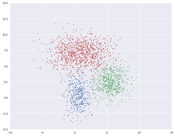
GMM的基本假设为数据是由几个不同的高斯分布的随机变量组合而成。如下图,我们就是用三个二维高斯分布生成的数据集。
在高斯混合模型中,我们需要估计每一个高斯分布的均值与方差。从最大似然估计的角度来说,给定某个有$n$个样本的数据集$X$,假如已知GMM中一共有$k$簇,我们就是要找到$k$组均值$\mu_1,\cdots,\mu_k$,$k$组方差$\sigma_1, \cdots, \sigma_k$来最大化以下似然函数$\mathcal L$
$$\mathcal L((\mu_1,\cdots,\mu_k), (\sigma_1, \cdots, \sigma_k);X).$$
这里直接计算似然函数比较困难,于是我们引入隐变量(latent variable),这里的隐变量就是每个样本属于每一簇的概率。假设$W$是一个$n\times k$的矩阵,其中$W_{i,j}$是第$i$个样本属于第$j$簇的概率。
在已知$W$的情况下,我们就很容易计算似然函数$\mathcal L_W$,
$$\mathcal{L}\_W((\mu\_1,\cdots,\mu\_k), (\sigma\_1, \cdots, \sigma\_k);X),$$
将其写成
$$\mathcal{L}\_W=\prod\_{i=1}^n\left(\sum\_{j=1}^k W\_{i,j}P(X\_i | \mu\_j, \sigma\_j)\right)$$
其中$P(X_i | \mu_j, \sigma_j)$是样本$X_i$在第$j$个高斯分布中的概率密度函数。
以一维高斯分布为例,
$$P(X_i | \mu_j, \sigma_j)=\frac{1}{\sqrt{2\pi \sigma_j^2}}e^{-\frac{(X_i-\mu_j)^2}{2\sigma_j^2}}$$
### 2. 最大期望算法(Expectation–Maximization, EM)
有了隐变量还不够,我们还需要一个算法来找到最佳的$W$,从而得到GMM的模型参数。EM算法就是这样一个算法。
简单说来,EM算法分两个步骤。
- **第一个步骤是E(期望),用来更新隐变量$W$;**
- **第二个步骤是M(最大化),用来更新GMM中各高斯分布的参量$\mu_j$, $\sigma_j$。**
然后重复进行以上两个步骤,直到达到迭代终止条件。
## 3. 具体步骤以及Python实现
完整代码在第4节。
首先,我们先引用一些我们需要用到的库和函数。
```python
import numpy as np
import matplotlib.pyplot as plt
from matplotlib.patches import Ellipse
from scipy.stats import multivariate_normal
plt.style.use('seaborn')
```
接下来,我们生成2000条二维模拟数据,其中400个样本来自$\mathcal N(\mu_1, \text{var}_1)$,600个来自$\mathcal N(\mu_2, \text{var}_2)$,1000个样本来自$\mathcal N(\mu_3, \text{var}_3)$
```python
# 第一簇的数据
num1, mu1, var1 = 400, [0.5, 0.5], [1, 3]
X1 = np.random.multivariate_normal(mu1, np.diag(var1), num1)
# 第二簇的数据
num2, mu2, var2 = 600, [5.5, 2.5], [2, 2]
X2 = np.random.multivariate_normal(mu2, np.diag(var2), num2)
# 第三簇的数据
num3, mu3, var3 = 1000, [1, 7], [6, 2]
X3 = np.random.multivariate_normal(mu3, np.diag(var3), num3)
# 合并在一起
X = np.vstack((X1, X2, X3))
```
数据如下图所示:
```python
plt.figure(figsize=(10, 8))
plt.axis([-10, 15, -5, 15])
plt.scatter(X1[:, 0], X1[:, 1], s=5)
plt.scatter(X2[:, 0], X2[:, 1], s=5)
plt.scatter(X3[:, 0], X3[:, 1], s=5)
plt.show()
```

### 3.1 变量初始化
首先要对GMM模型参数以及隐变量进行初始化。通常可以用一些固定的值或者随机值。
`n_clusters`是GMM模型中聚类的个数,和K-Means一样我们需要提前确定。这里通过观察可以看出是`3`。(拓展阅读:[如何确定GMM中聚类的个数?](http://sofasofa.io/forum_main_post.php?postid=1001676))
`n_points`是样本点的个数。
`Mu`是每个高斯分布的均值。
`Var`是每个高斯分布的方差,为了过程简便,我们这里假设协方差矩阵都是对角阵。
`W`是上面提到的隐变量,也就是每个样本属于每一簇的概率,在初始时,我们可以认为每个样本属于某一簇的概率都是$1/3$。
`Pi`是每一簇的比重,可以根据`W`求得,在初始时,`Pi = [1/3, 1/3, 1/3]`
```python
n_clusters = 3
n_points = len(X)
Mu = [[0, -1], [6, 0], [0, 9]]
Var = [[1, 1], [1, 1], [1, 1]]
Pi = [1 / n_clusters] * 3
W = np.ones((n_points, n_clusters)) / n_clusters
Pi = W.sum(axis=0) / W.sum()
```
### 3.2 E步骤
E步骤中,我们的主要目的是更新`W`。第$i$个变量属于第$m$簇的概率为:
$$W\_{i,m}=\frac{\pi\_j P(X\_i|\mu\_m, \text{var}\_m)}{\sum\_{j=1}^3 \pi\_j P(X\_i|\mu\_j, \text{var}\_j)}$$
根据$W$,我们就可以更新每一簇的占比$\pi_m$,
$$\pi\_m=\frac{\sum\_{i=1}^n W\_{i,m}}{\sum\_{j=1}^k\sum\_{i=1}^n W\_{i,j}}$$
```python
def update_W(X, Mu, Var, Pi):
n_points, n_clusters = len(X), len(Pi)
pdfs = np.zeros(((n_points, n_clusters)))
for i in range(n_clusters):
pdfs[:, i] = Pi[i] * multivariate_normal.pdf(X, Mu[i], np.diag(Var[i]))
W = pdfs / pdfs.sum(axis=1).reshape(-1, 1)
return W
def update_Pi(W):
Pi = W.sum(axis=0) / W.sum()
return Pi
```
以下是计算对数似然函数的`logLH`以及用来可视化数据的`plot_clusters`。
```python
def logLH(X, Pi, Mu, Var):
n_points, n_clusters = len(X), len(Pi)
pdfs = np.zeros(((n_points, n_clusters)))
for i in range(n_clusters):
pdfs[:, i] = Pi[i] * multivariate_normal.pdf(X, Mu[i], np.diag(Var[i]))
return np.mean(np.log(pdfs.sum(axis=1)))
def plot_clusters(X, Mu, Var, Mu_true=None, Var_true=None):
colors = ['b', 'g', 'r']
n_clusters = len(Mu)
plt.figure(figsize=(10, 8))
plt.axis([-10, 15, -5, 15])
plt.scatter(X[:, 0], X[:, 1], s=5)
ax = plt.gca()
for i in range(n_clusters):
plot_args = {'fc': 'None', 'lw': 2, 'edgecolor': colors[i], 'ls': ':'}
ellipse = Ellipse(Mu[i], 3 * Var[i][0], 3 * Var[i][1], **plot_args)
ax.add_patch(ellipse)
if (Mu_true is not None) & (Var_true is not None):
for i in range(n_clusters):
plot_args = {'fc': 'None', 'lw': 2, 'edgecolor': colors[i], 'alpha': 0.5}
ellipse = Ellipse(Mu_true[i], 3 * Var_true[i][0], 3 * Var_true[i][1], **plot_args)
ax.add_patch(ellipse)
plt.show()
```
### 3.2 M步骤
M步骤中,我们需要根据上面一步得到的`W`来更新均值`Mu`和方差`Var`。
`Mu`和`Var`是以`W`的权重的样本`X`的均值和方差。
因为这里的数据是二维的,第$m$簇的第$k$个分量的均值,
$$\mu\_{m,k} = \frac{\sum\_{i=1}^n W\_{i,m}X\_{i,k}}{\sum\_{i=1}^n W\_{i,m}}$$
第$m$簇的第$k$个分量的方差,
$$\text{var}\_{m,k} = \frac{\sum\_{i=1}^n W\_{i,m}(X\_{i,k} - \mu\_{m,k})^2}{\sum\_{i=1}^n W\_{i,m}}$$
以上迭代公式写成如下函数`update_Mu`和`update_Var`。
```python
def update_Mu(X, W):
n_clusters = W.shape[1]
Mu = np.zeros((n_clusters, 2))
for i in range(n_clusters):
Mu[i] = np.average(X, axis=0, weights=W[:, i])
return Mu
def update_Var(X, Mu, W):
n_clusters = W.shape[1]
Var = np.zeros((n_clusters, 2))
for i in range(n_clusters):
Var[i] = np.average((X - Mu[i]) ** 2, axis=0, weights=W[:, i])
return Var
```
### 3.3 迭代求解
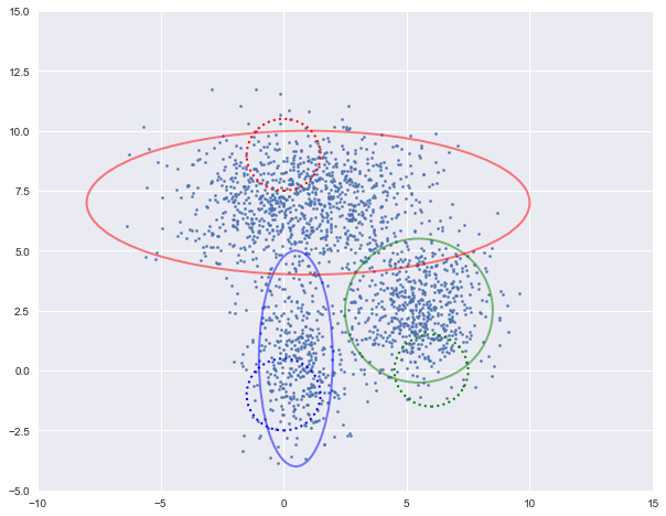
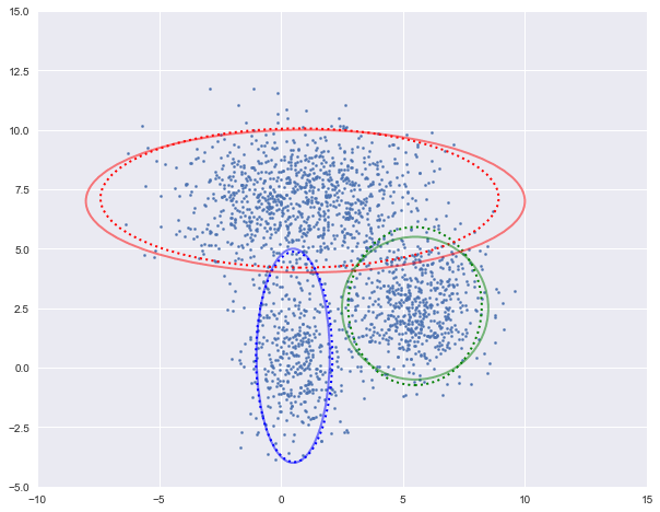
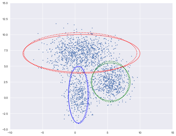
下面我们进行迭代求解。
图中实现是真实的高斯分布,虚线是我们估计出的高斯分布。可以看出,经过5次迭代之后,两者几乎完全重合。
```python
loglh = []
for i in range(5):
plot_clusters(X, Mu, Var, [mu1, mu2, mu3], [var1, var2, var3])
loglh.append(logLH(X, Pi, Mu, Var))
W = update_W(X, Mu, Var, Pi)
Pi = update_Pi(W)
Mu = update_Mu(X, W)
print('log-likehood:%.3f'%loglh[-1])
Var = update_Var(X, Mu, W)
```
log-likehood:-8.054
log-likehood:-4.731

log-likehood:-4.729

log-likehood:-4.728
log-likehood:-4.728
## 4. 完整代码
```python
import numpy as np
import matplotlib.pyplot as plt
from matplotlib.patches import Ellipse
from scipy.stats import multivariate_normal
plt.style.use('seaborn')
# 生成数据
def generate_X(true_Mu, true_Var):
# 第一簇的数据
num1, mu1, var1 = 400, true_Mu[0], true_Var[0]
X1 = np.random.multivariate_normal(mu1, np.diag(var1), num1)
# 第二簇的数据
num2, mu2, var2 = 600, true_Mu[1], true_Var[1]
X2 = np.random.multivariate_normal(mu2, np.diag(var2), num2)
# 第三簇的数据
num3, mu3, var3 = 1000, true_Mu[2], true_Var[2]
X3 = np.random.multivariate_normal(mu3, np.diag(var3), num3)
# 合并在一起
X = np.vstack((X1, X2, X3))
# 显示数据
plt.figure(figsize=(10, 8))
plt.axis([-10, 15, -5, 15])
plt.scatter(X1[:, 0], X1[:, 1], s=5)
plt.scatter(X2[:, 0], X2[:, 1], s=5)
plt.scatter(X3[:, 0], X3[:, 1], s=5)
plt.show()
return X
# 更新W
def update_W(X, Mu, Var, Pi):
n_points, n_clusters = len(X), len(Pi)
pdfs = np.zeros(((n_points, n_clusters)))
for i in range(n_clusters):
pdfs[:, i] = Pi[i] * multivariate_normal.pdf(X, Mu[i], np.diag(Var[i]))
W = pdfs / pdfs.sum(axis=1).reshape(-1, 1)
return W
# 更新pi
def update_Pi(W):
Pi = W.sum(axis=0) / W.sum()
return Pi
# 计算log似然函数
def logLH(X, Pi, Mu, Var):
n_points, n_clusters = len(X), len(Pi)
pdfs = np.zeros(((n_points, n_clusters)))
for i in range(n_clusters):
pdfs[:, i] = Pi[i] * multivariate_normal.pdf(X, Mu[i], np.diag(Var[i]))
return np.mean(np.log(pdfs.sum(axis=1)))
# 画出聚类图像
def plot_clusters(X, Mu, Var, Mu_true=None, Var_true=None):
colors = ['b', 'g', 'r']
n_clusters = len(Mu)
plt.figure(figsize=(10, 8))
plt.axis([-10, 15, -5, 15])
plt.scatter(X[:, 0], X[:, 1], s=5)
ax = plt.gca()
for i in range(n_clusters):
plot_args = {'fc': 'None', 'lw': 2, 'edgecolor': colors[i], 'ls': ':'}
ellipse = Ellipse(Mu[i], 3 * Var[i][0], 3 * Var[i][1], **plot_args)
ax.add_patch(ellipse)
if (Mu_true is not None) & (Var_true is not None):
for i in range(n_clusters):
plot_args = {'fc': 'None', 'lw': 2, 'edgecolor': colors[i], 'alpha': 0.5}
ellipse = Ellipse(Mu_true[i], 3 * Var_true[i][0], 3 * Var_true[i][1], **plot_args)
ax.add_patch(ellipse)
plt.show()
# 更新Mu
def update_Mu(X, W):
n_clusters = W.shape[1]
Mu = np.zeros((n_clusters, 2))
for i in range(n_clusters):
Mu[i] = np.average(X, axis=0, weights=W[:, i])
return Mu
# 更新Var
def update_Var(X, Mu, W):
n_clusters = W.shape[1]
Var = np.zeros((n_clusters, 2))
for i in range(n_clusters):
Var[i] = np.average((X - Mu[i]) ** 2, axis=0, weights=W[:, i])
return Var
if __name__ == '__main__':
# 生成数据
true_Mu = [[0.5, 0.5], [5.5, 2.5], [1, 7]]
true_Var = [[1, 3], [2, 2], [6, 2]]
X = generate_X(true_Mu, true_Var)
# 初始化
n_clusters = 3
n_points = len(X)
Mu = [[0, -1], [6, 0], [0, 9]]
Var = [[1, 1], [1, 1], [1, 1]]
Pi = [1 / n_clusters] * 3
W = np.ones((n_points, n_clusters)) / n_clusters
Pi = W.sum(axis=0) / W.sum()
# 迭代
loglh = []
for i in range(5):
plot_clusters(X, Mu, Var, true_Mu, true_Var)
loglh.append(logLH(X, Pi, Mu, Var))
W = update_W(X, Mu, Var, Pi)
Pi = update_Pi(W)
Mu = update_Mu(X, W)
print('log-likehood:%.3f'%loglh[-1])
Var = update_Var(X, Mu, W)
```
<ul class="pager">
<li class="next"><a href="../../tutorials.php"><b><i class="fa fa-graduation-cap" aria-hidden="true"></i>&nbsp; 学完咯!</b></a></li>
</ul>